Introduction

Canal preparation is one of the major steps in root canal treatment and directly related to subsequent disinfection and obturation. In recent years, the advent of Ni–Ti rotary root canal preparation techniques like ProFile (Dentsply Maillefer, Ballaigues, Switzerland) or Lightspeed (Lightspeed Inc, San Antonio TX, USA), has altered the perception of canal instrumentation. Consequently, the performance of these rotary techniques requires close evaluation.

Several publications discussed aspects of root canal preparations using plastic blocks (Thompson & Dummer 1997, Bryant et al. 1998a, 1998b). Whilst having the advantage of standardized dimensions, plastic blocks lack the material qualities of human dentine. Furthermore, canal curvature as simulated in plastic blocks is only two-dimensional. Another in vitro approach used cross-sections of human root canals to determine the amount of dentine removed and cross-sectional canal transportation (Bramante et al. 1987, Portenier et al. 1998). Recently, microcomputed tomography (μCT) has evolved as a promising tool in endodontic research (Bjørndal et al. 1999, Rhodes et al. 1999).

Earlier investigations using m CTs were hampered by insufficient resolution (Gambill et al. 1996) or projection errors (Nielsen et al. 1995). Recently, more suitable measurement software has became available on a prototype basis, allowing evaluation of three-dimensionally matched specimens before and after preparation (Peters et al. 2000a, 2000b). In a pilot study, sufficient accuracy of the method was demonstrated (Peters et al. 2000a). Furthermore, algorithms allowed measurement of basic geometrical parameters such as volume and surface area as well as additional descriptors of canal shape such as Structure Model Index (SMI) and thickness (Peters et al. 2000c). Nevertheless, due to the prolonged scanning and reconstruction times (up to 4 h per specimen), the methods of earlier studies were unbalanced and evaluated too few specimens (Nielsen et al. 1995, Rhodes et al. 1999, Peters et al. 2000b).

Different instrument geometry will produce canals with different shapes. Different approaches to root canal preparation, i.e. relatively large apical preparations using the Lightspeed system versus small and more tapered preparations achieved using GT rotary instruments (Dentsply Maillefer) might be mirrored in three-dimensional canal geometry.

Therefore, the aim of this study was to assess the effects of four root canal preparation techniques on canal volume and surface area using three-dimensionally reconstructed root canals in extracted human maxillary molars. Furthermore, μCT data were used to describe additional morphometric parameters related to those different preparation techniques. Finally, an attempt was made to quantify canal transportation three-dimensionally.

Materials and methods

Preparation of specimens

A total of 40 three-rooted maxillary molars were selected from a pool of extracted teeth which were stored in 0.1% thymol solution until used. Access cavities were prepared and ISO 10 K-Files (Dentsply Maillefer, Ballaigues, Switzerland) were inserted into the canals so that their tips were just visible at the apical foramina. With the files in place, the outer root surface from the apices to the cemento-enamel junctions was sealed using a dentine bonding system (Syntac Classic; Vivadent, Schaan, Liechtenstein). The bonding resin was cured for 1 min using an Optilux 500 curing lamp (Demetron Res., Danbury, CT, USA). The specimens were then mounted on SEM stubs (Spec. 109Pb, Laubscher, Täuffelen, Switzerland) using custom-made moulds with an internal diameter of 15 mm into which self-curing resin (Stycast, Emerson & Cuming, Oevel, Belgium) was poured. Finally, a specially designed attachment was fitted to ensure subsequent precise repositioning of the specimens into the scanning system (Fig. 1).

The specimens were divided into four groups of 10. Of the 120 canals, 30 canals each were assigned for preparation by either Ni–Ti K-Files (Dentsply Maillefer), Lightspeed (Lightspeed Inc), ProFile .04 Instruments (Dentsply Maillefer) and GT-Rotaries (Dentsply Maillefer). Care was taken to divide the specimens equally into the four groups with respect to canal curvatures. Curvatures were judged from digital radiographs (Digora, Soredex, Helsinki, Finland) and determined quantitatively using μCT data (see below).

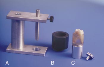
Figure 1. Apparatus used to embed and reposition the specimens. A) Alignment tool, B) mould, C) specimen mounted on connector and SEM stub.

Root canal preparation

All canals were first stepped-down using Gates-Glidden burs (Dentsply Maillefer) nos. 4 through 1 sequentially. Each bur was carried about 1 mm into the root canals, so that the coronal 4 mm were prepared. Working lengths were determined during the canal preparation at an appropriate point for the specific preparation technique used and were verified using digital radiographs. The canals were copiously irrigated throughout the stepdown using 2.5% NaOCl.

No attempt was made to prepare the second mesiobuccal canals in this study, because they did not always present as separate canals along the entire length of the root.

Canal preparation was done by two of the authors (O. P., K. S.). Care was taken to distribute specimens evenly between the two operators, i.e. each operator instrumented an equal number of specimens with the four canal preparation techniques.

GT rotary instruments Canals assigned to group 1 were prepared with GT rotary instruments in a crowndown fashion after preflaring with a no. 35 (.12 taper). The canals were instrumented to an apical size no. 20 with tapers varying from .06 for most of the mesio- and disto-buccal and .08 or .10 for the palatal canals and recapitulated using the master apical rotary. Working lengths in group 1 were set 0.5 mm short of the portal of exit.

Ni–Ti K-Files In group 2, Ni–Ti K-Files were used in a balanced-force motion. These canals were stepped-back to a size 80 file and recapitulated with the master apical file after completing the preparation. Apical stops for the mesio-buccal and disto-buccal canals were prepared to size 40, whilst the apical stops for the palatal canals were shaped to size 45. Working lengths were set to be 1 mm short of the main portal of exit.

Lightspeed Canals assigned to group 3 were prepared with Lightspeed instruments used strictly according to the manufacturer’s instructions. These canals were stepped-back to a size 80, 90 or 100 instrument and recapitulated with the master apical rotary after completing the preparation. Apical stops for the mesio-buccal and disto-buccal canals were prepared to size 40, whilst the apical stops for the palatal canals were shaped to size 45. Working lengths were set to be 1 mm short of the main portal of exit.

ProFile Canals in group 4 were prepared in a crowndown fashion using ProFile .04 instruments from sizes no. 60 through no. 15. Apical stops were shaped and the canals then stepped-back to size 60. Again, the preparation was concluded by recapitulating with the master apical rotary. Apical stops for the mesio-buccal and disto-buccal canals were prepared to size 40, whilst the apical stops for the palatal canals were shaped to size 45. Working lengths were set to be 1 mm short of the main portal of exit.

All canals in the four groups were copiously irrigated after each instrument alternating between 2.5% NaOCl and 17% EDTA.

Micro CT measurements and evaluations

A protototype microcomputed tomography system with an isotropic nominal resolution of 19.6 m m was used (Scanco Medical, Bassersdorf, Switzerland) at 60 kV to scan the specimens before and after preparation. Typically, 200–340 slices with a voxel size of

39.2 × 39.2 × 39.2 μm were scanned with each scanning procedure requiring about 20 min per stack (256 slices). For long specimens, two stacks of slices were scanned and combined. An additional time of 2 h was required for segmentation and reconstruction of the data.

Volumes of interest were selected extending from the furcation region to the apex of the roots. The original grayscale images were then processed with a slight Gaussian low-pass filtration for noise reduction and a fixed segmentation threshold to separate root dentine from the root canals. These procedures produced binary images of the root canals. The high contrast of dentine to the root canals filled with thymol or air yielded excellent segmentation of the specimens. Although the special mounting device ensured almost exact repositioning of the samples (error <2 voxel) with minimal rotational error (<1°), the precision was perfected by superimposing two sets of segmented root canals over each other. Then, by varying the relative translation in all three directions, the best superimposition of the outer root contour was automatically detected with a precision better than 1 voxel. Visualization of reconstructed images (Fig. 2) was carried out using volume rendering (VGL Image Max 2.0, Volume Graphics, Heidelberg, Germany) and Quick-Time movies (Apple, Cupertino, CA, USA).

Subsequently, matched root canals were evaluated as follows: volumes and surface areas of the root canals were determined from triangulated data using the ‘Marching Cubes’ algorithm. Increases in volume and surface area were calculated by subtracting the scores for the treated canals from those recorded for the untreated counterparts. Triangulated data were also used to determine Structure Model Indices (SMI) and ‘thicknesses’ of the canals. The applicability in endodontics of these indices which had been originally developed to characterize trabecular bone has been previously described in detail (Peters et al. 2000c). In brief, the SMI characterizes a structure as being ribbon-shaped versus cylindrical and is expressed in arbitrary units. The range is from 0 (= parallel flat planes) to 4 (= an ideal ball). The term ‘thickness’ refers to the maximal diameter of balls inscribed into the volume of interest. Furthermore, the conicity of the canals was calculated by relating thicknesses to the lengths of the canals.

Images of the untreated and the instrumented canals were not superimposed when using the μCT technique to assess volume, surface, SMI and thickness. These parameters were evaluated separately for the exactly matched volumes of interest. However, exact superimposition had to be accomplished, before and after canal preparation, to obtain reproducible results for centres of gravity (CoG) because the data sets were then compared voxel by voxel in each slice.

Each slice was defined by a series of coordinated data for the x-, y- and z-axes. The first two axes were parallel to the slice, whilst the z-axis is at right angles to each slice. CoGs of the canals, calculated for each slice, were connected along the z-axis by a fitted line. This fitted line was analysed mathematically to determine canal curvature as the second derivative. Furthermore, average canal transportations were calculated by comparing CoGs before and after treatment for the apical, middle and coronal thirds of the canals. Canal transportation, in μm, was expressed in relation to the coordinates and also correlated to the canals’ main curves.

Finally, matched images of the surface area of the canals, before and after preparation, were examined to evaluate the amount of surface area instrumented. It was assumed that surface voxels remaining in the same place, before and after treatment, represented uninstrumented parts of the canal walls. The amount of instrumented surface could be calculated by subtracting the number of static surface voxels from the total number of surface voxels. All measurements were performed using proprietary software run on an Open VMS platform (DEC Compaq, Zürich, Switzerland).

Statistical analysis

Mean scores were calculated, and differences between means of the groups investigated were analysed statistically. Initial test indicated that data were normally distributed. Subsequently, t-tests, ANOVA s and Scheffe’s tests from the Statview 4.02 statistics package (Abacus, Berkeley, CA, USA) were run on a Macintosh PC.

Results

Uninstrumented specimens

Volume rendering revealed detailed images of outer root contours, as well as root canal systems (Fig. 2). Gross canal anatomy was studied using volume rendered images of isolated root canals (Figs 2, 3a, 4a). Palatal and disto-buccal roots were found to have one root canal in all cases. In contrast, mesio-buccal canals presented with complicated canal systems which were further classified according to Weine (Weine 1996). The majority of mb canals were classified as type 2 (19/40) and 14/40 were type 3. Three and four canals were classified as type 1 and 4, respectively. In total, 37 cases (92.5%) had a second mesio-buccal (mb2) canal present.

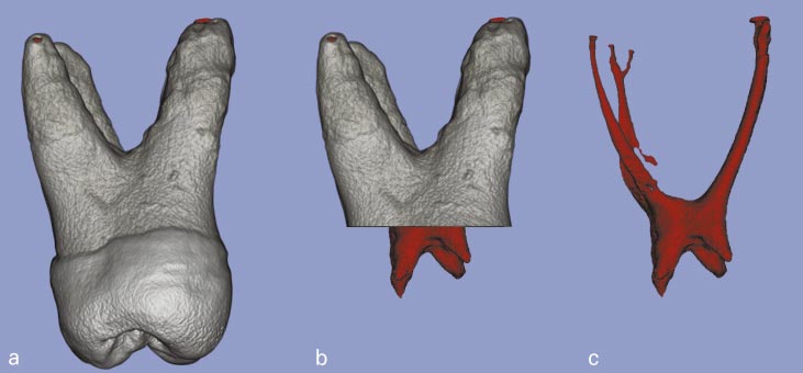
Figure 2. Volume rendered image of external and internal morphology of scanned maxillary molar. Viewed from left to right are: (a) external view of a specimen, (b) image after removal of coronal hard structure, (c) pulp morphology with mb2 canal and apical furcation.

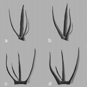
Figure 3. Typical examples of effects of GT File preparation on root canal anatomy illustrated by μCT images. Mesio-buccal canal system classified as class 3. a, b) clinical projection before and after instrumentation. c, d) mesio-distal projection before and after instrumentation.

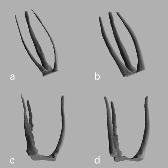
Figure 4. Typical examples of effects of ProFile. 04 preparation on root canal anatomy illustrated by μCT images. Mesio-buccal canal system classified as class 2. a, b) clinical projection before and after instrumentation. c, d) mesio-distal projection before and after instrumentation.

Table 1 Morphometric data determined for untreated maxillary root canalsa (means ± SD, n = 40)

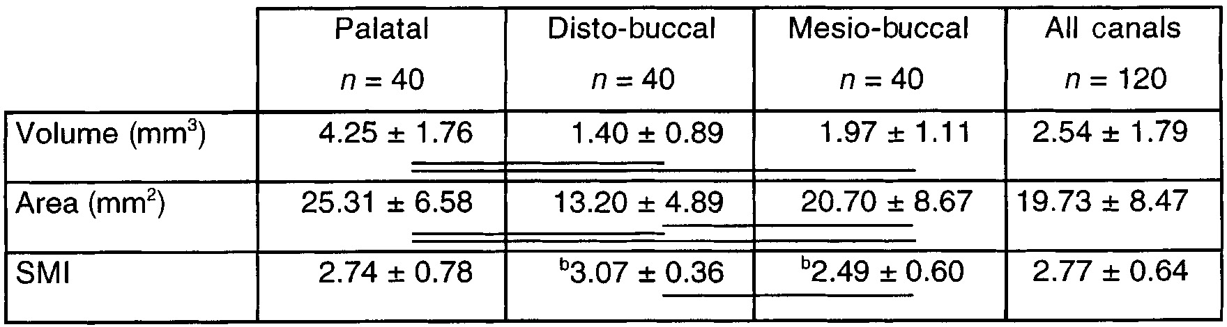
Significant differences are denoted by horizontal bars (Factorial ANOVA, P < 0.001).

aAreas of interest extended from furcations to portals of exit. bP < 0.01.

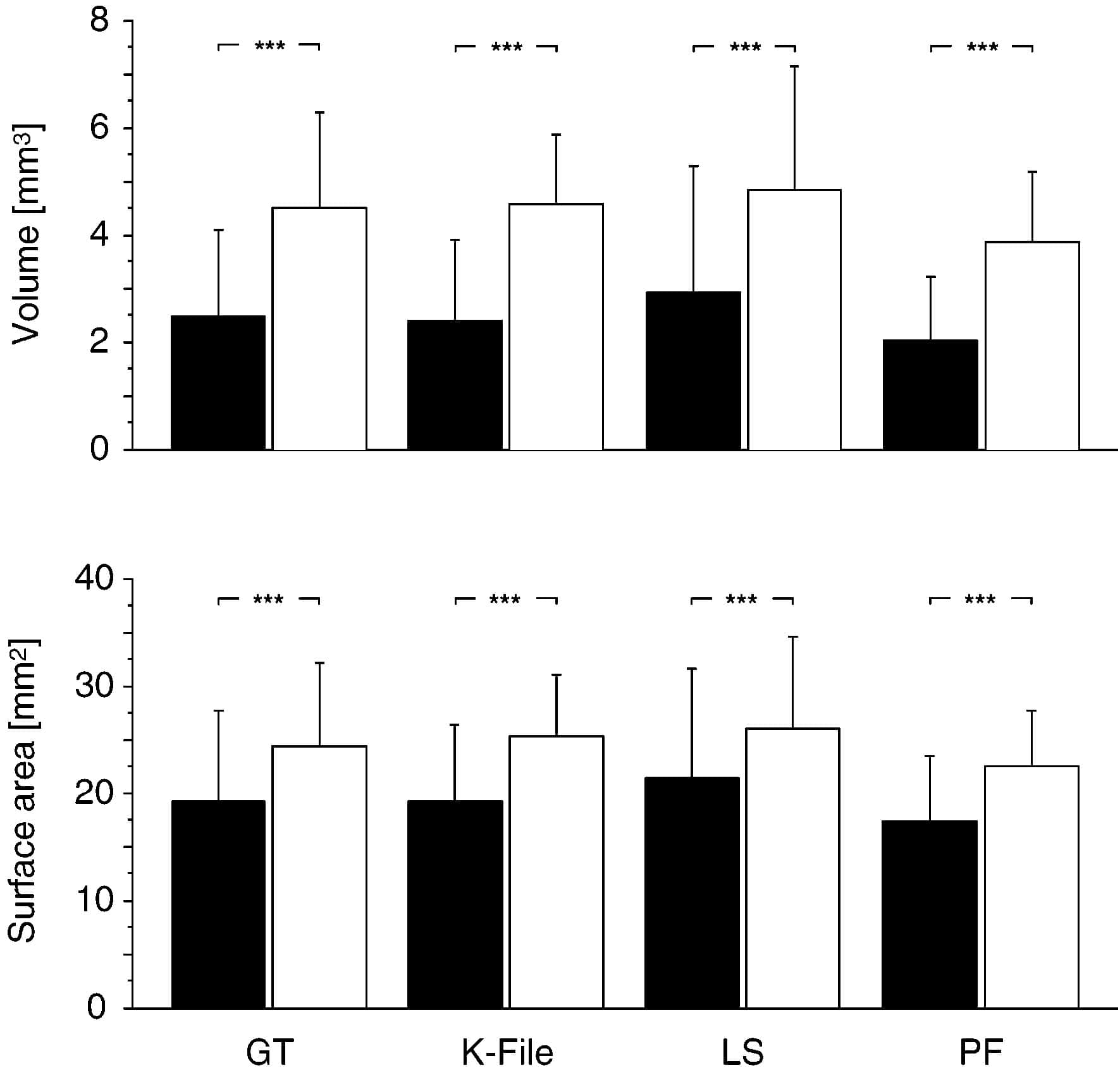
Figure 5. Bar diagrams illustrating canal volumes and surface areas (means ± SD) related to instrument type. Filled bars indicate scores before, open bars scores after preparation. Significant differences (P < 0.001, paired t-test) are indicated by asterisks. Areas of interest extended from furcation to portal of exit. No significant differences between experimental groups before and after preparation (ANOVA).

Effect of instrumentation on basic canal geometry

The effect of root canal preparation gave rise to substantial changes in gross canal anatomy, depending on the type of instrument used (Figs 3 and 4). Canals prepared with GT rotary instruments had a marked taper (Fig. 3b,d) whereas the three other techniques produced more parallel canal walls and blunt apical preparations (Fig. 4b,d). Quantitative analysis revealed that instrumentation resulted in mean increases in canal volume ranging between 1.85 and 2.18 mm3 (Fig. 5). Surface areas were increased after instrumentation in the vast majority of the cases (Fig. 5); these gains were statistically highly significant.

However, a minute decrease in canal areas was noted in three palatal canals, in which also a substantial amount of irregular hard tissue had been observed preoperatively. These three cases were excluded from further analyses.

ANOVA indicated that there were no statistically significant differences between the four experimental groups with respect to changes in volume and surface areas. By contrast, significant differences were noted when grouping was made with respect to canal type (Table 2). Similar results were obtained for differences in SMI and thickness (Fig. 6, Table 2). However, canals prepared with GT rotary instruments had a significantly more distinct conicity than canals prepared with the three other techniques (P < 0.001, Fig. 6). The conicity of a GT prepared canal was similar to a .08 taper, whereas the other three techniques rendered canals resembling .06 tapers. Furthermore, canal curvatures were found to change in varying degrees after canal instrumentation (Table 3). Overall, canal preparation led to a loss of canal curvature. The relative degrees of canal straightening were 11.7 ± 18.2, 19.4 ± 16.1, 14.2 ± 20.5 and 13.8 ± 20.1% for GT File, Hand instruments, Lightspeed and ProFile, respectively. Whilst there were significant differences with respect to canal type (P < 0.001, Table 3), again, no such differences were found between instrument types.

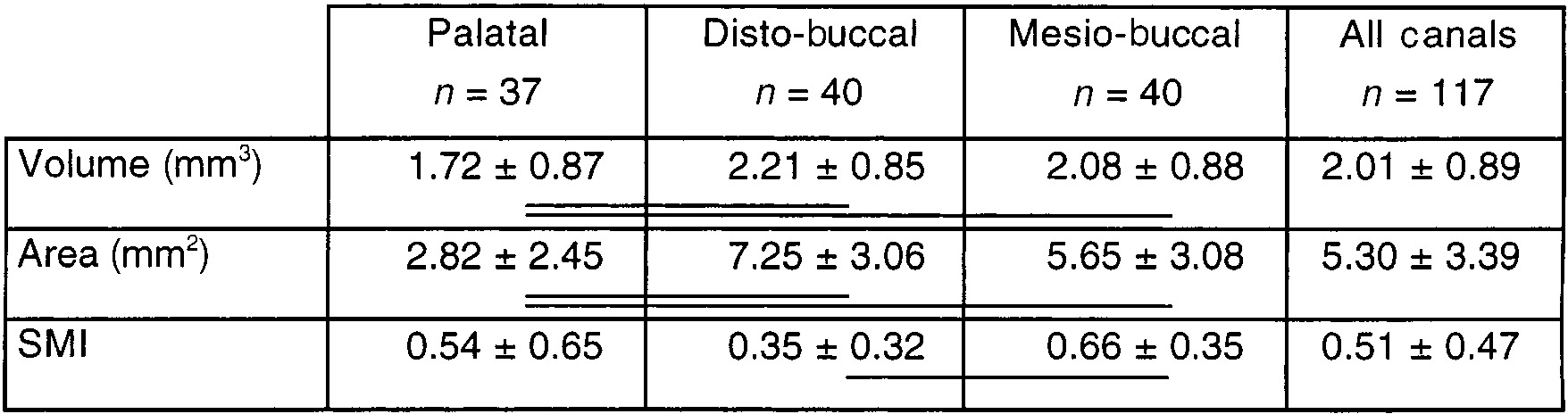
Table 2 Changes in canal volume, surface area and SMI after preparationa (means ± SD)

Significant differences are denoted by horizontal bars (Factorial ANOVA, P < 0.001).

aGrouping with respect to canal type.

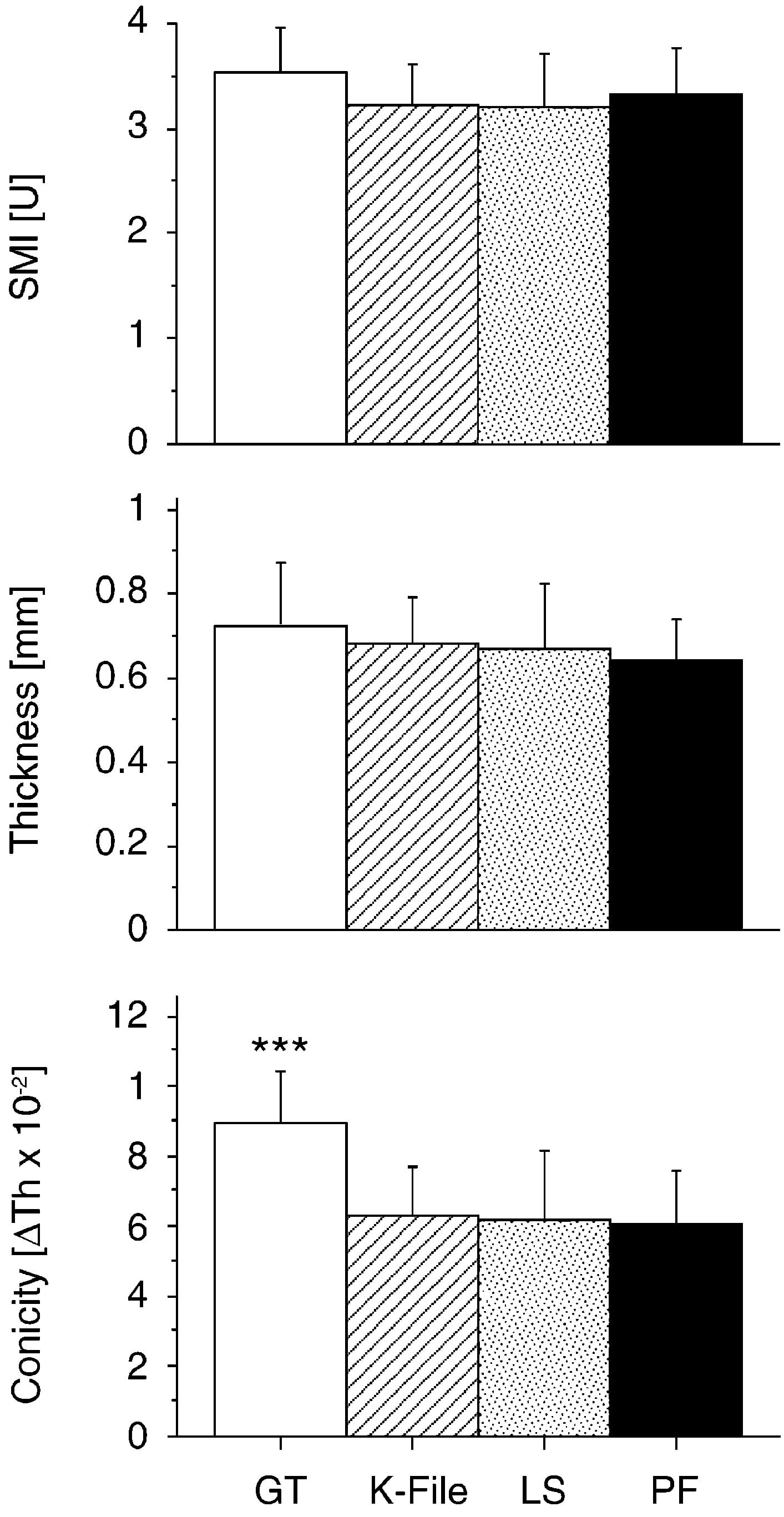
Figure 6. Bar diagrams showing postoperative scores for Structure Model Indices, thickness and conicity (means ± SD) grouped with respect to instrument type. Significant difference between groups is marked by asterisk (P < 0.001, ANOVA).

Table 3 Relative degree of canal straighteninga (means ± SD, n = 40)

Significant differences are denoted by horizontal bars (Factorial ANOVA, P < 0.001).

aGrouping with respect to canal type.

bStraightening expressed as difference in canal curvature in relation to initial scores.

Canal transportation after instrumentation

Figure 7 illustrates the amount of canal transportation, expressed as centre of gravity (CoG) shift. Overall, mean canal transportations were 123.66 ± 84.2, 89.81 ± 70.87 and 97.72 ± 99.13 μm for the coronal, middle and apical root canal thirds, respectively. Furthermore, GT rotary instruments and Lightspeed instruments had significantly larger values in the coronal third, whilst no such differences were noted with hand instrumentation and ProFile .04 (Fig. 7). However, 32 cases were found in which the amount of transportation exceeded 200 μm and those accounted for 12, seven, six and seven specimens instrumented with GT, K-Files, Lightspeed and ProFile .04, respectively.

No specific pattern was found with respect to the direction of canal transportation versus instrument type and canal area (Table 4). Whilst there was a similar distribution between canals transported outwards and inwards in the coronal and middle part of the canals, the vast majority of the specimens showed an outwards transportation in the apical third. However, 43.3% and 33.3% out of the Lightspeed–prepared canals, were transported inwards apically and outwards coronally, respectively.

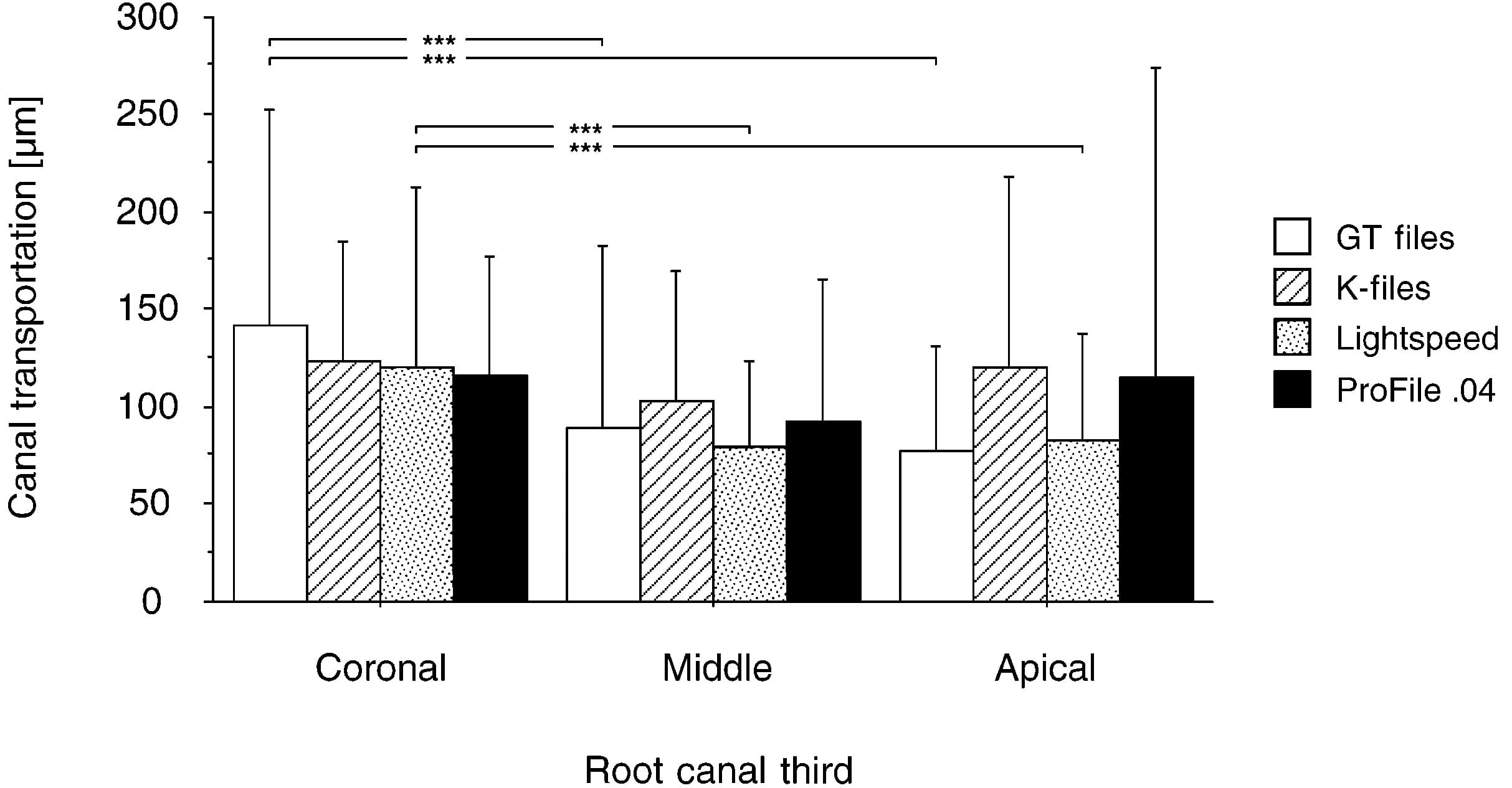
Figure 7. Bar diagram illustrating canal transportation (means ± SD) in the three root levels analysed. Significant differences between groups (P < 0.001, paired t-test) are marked by asterisks.

Table 4 Direction of canal transportation with respect to the canal’s main curve

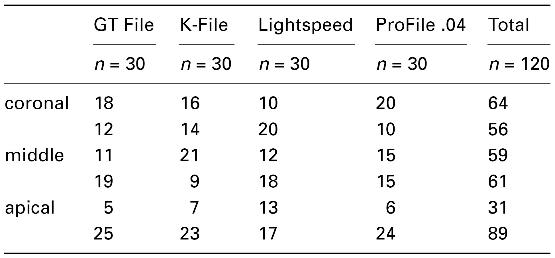
aNumbers of canals with transportation inwards (upper lines) and outwards (lower lines) are indicated.

Instrumented canal surface area

Subtraction of three-dimensionally reconstructed images of uninstrumented and instrumented specimens slice per slice rendered the surface area with changes less than 1 voxel. Table 5 shows the absolute and relative amount of static voxels before and after preparation, indicating that approximately 35–40% of the root canal surface remained in the same position. However, a wide range of unchanged surfaces (3–89%) was recorded. Although specimens prepared with GT Files had the largest mean amount of static voxels, no statistically significant differences were noted between groups 1–4.

Table 5 Numbers and percentages of static voxels recorded by superimposing matched images, before and after preparation

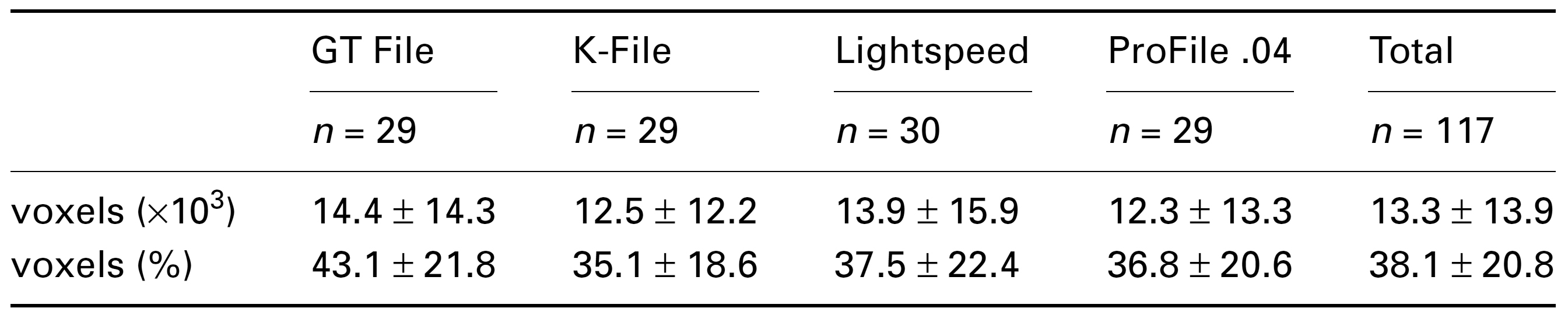
aRelative findings are expressed as percentages calculated in relation to surface areas after preparation. No significant differences between groups.

Effect of operator variability on registered variables

Equal numbers of specimens were instrumented by the two main authors (O. P. and K. S.). Comparing these two groups, no differences were seen with respect to all analysed variables (P > 0.5, ANOVA).

Discussion

The present study evaluated root canal geometry using high-resolution tomography or μCT. Recently this technique has evolved into an exciting tool for experimental endodontology (Rhodes et al. 1999). Whilst there have been some attempts in the past to use μCT to compare different root canal preparation techniques, these studies had small sample sizes or large spatial resolutions (Nielsen et al. 1995, Gambill et al. 1996, Dowker et al. 1997). Furthermore, three-dimensional visualization alone does not use the full potential of μCT techniques, which can also be used for quantitative evaluation of objects of interest.

Spatial resolution has improved continuously over time from 127μm (Nielsen et al. 1995) to 33 mm (Bjørndal et al. 1999). However, improvements in resolution will be reflected in a long scanning time which is added to an already long reconstruction period. This holds especially for fan beam systems which require one turn of the object turntable per CT slice. In contrast, cone beam projection allows for faster scanning times (Davis & Wong 1996, Rhodes et al. 1999). There is, however, a projection error inherent to cone beam technology which can be compensated by adequate reconstruction algorithms (Davis & Wong 1996, Rhodes et al. 1999). In this study, a stacked fan beam projection was used which allowed scanning of the entire object in one single sweep. This step reduced scanning time to approximately 20 min per stack.

As hardware improved, new measurement algorithms were developed in order to three-dimensionally describe objects of interest metrically (Hildebrand & Rüegsegger 1997a, 1997b). The applicability of these indices that were designed primarily to describe cancellous bone to endodontics has been demonstrated recently (Peters et al. 2000c). Furthermore, the methods used in the current study were judged to be accurate and reproducible within the limits of the system (Peters et al. 2000a, 2000c).

However, it is important to know the possible sources of errors to avoid overinterpretation of three-dimensionally reconstructed images (Mol 1999). The segmentation process by itself tends to overemphasize sharp edges as there is a ‘yes or no’ decision. For root canals, this means if a canal is smaller than the resolution, no canal will be seen in the reconstructed image. Furthermore, any details of surfaces will appear sharper than in reality (Davis & Wong 1996). Therefore, quantitative assessments of three-dimensional reconstructed images should to be interpreted carefully (Dowker et al. 1997). Nevertheless, root canals present steep attenuation gradients which makes segmentation robust. Under the conditions of the current study, the difference between attenuation coefficients of dentine and the root canal filled with air or fluids was approximately 17 cm–1.

The three-dimensionally reconstructed images of canal systems in the current study were used to assess the morphology of mesio-buccal root canal systems. The vast majority of specimens had a second canal present. The proportion of 92.5% corresponds to that reported in a recent clinical study (Stropko 1999) but is higher than that stated in earlier in vitro studies (Weine et al. 1969). However, clinical X-ray projection and clinical expertise cannot detail the three-dimensional canal anatomy comparable to μCT.

The effect of canal instrumentation was analysed using a set of variables comprising canal volume and surface area, Structure Model Index, thickness and conicity. All these measures are mean values over the entire canal length and are therefore overall measures of canal anatomy (Peters et al. 2000c). Root canal instrumentation resulted in significant gains in canal volume and surface area with no apparent difference between the four preparation techniques investigated. This finding is in agreement with earlier studies stating mean volume gains of 3.725 mm3 (Rhodes et al. 1999) and between 26 and 58% (Nielsen et al. 1995). However, there is no consistent definition of boundaries of the volume of interest investigated.

The quantitative description of cross-sectional geometry of root canals has been attempted earlier using fractal geometry (Bjørndal et al. 1999). This procedure compares two outlines such as the outer root contour and the root canal cross-section but the current study concentrated on root canal geometry and therefore used fully three-dimensional measures such as SMI and thickness (Hildebrand & Rüegsegger 1997a, 1997b, Peters et al. 2000c).

Within the pulp tissue, several small irregular mineralized particles were found and their surface areas were added to the total surface area of the respective root canals. Removal of these particles during preparation resulted in minute decreases in surface areas, despite the canals having been enlarged. Therefore, these cases were excluded from the subsequent analyses. The same effect may have accounted for decreased surface areas in an earlier μCT study (Nielsen et al. 1995).

There were also no significant differences between the experimental groups with respect to SMI and thickness. In contrast, in all cases significant differences were demonstrated between canal types. This corroborates earlier findings indicating that individual canal anatomy can have a great impact on postoperative canal geometry (Peters et al. 2000b). Nevertheless, GT Files differed from the three other techniques in the production of canals of significantly greater conicity. However, further studies with μCTs are required to detail the effects of different preparation techniques on the apical portions of root canals.

The four instrumentation techniques investigated had comparable scores for canal transportation in the coronal and middle portion of the canals. Similar results were obtained in recent studies comparing Lightspeed versus Ni–Ti K-Files and stainless steel versus Ni–Ti K-Files using the Bramante technique (Porto Carvalho et al. 1999, Deplazes et al. 2000). The relatively large and uniform scores (mean values of approximately 130–150 mm) for canal transportation in the coronal third might be explained by using Gates Glidden burs in a step-down procedure as a prerequisite in all techniques in this study. Apically, the lowest canal transportation scores resulted when GT Files or Lightspeed instruments were used. Again, similar findings have been obtained in earlier studies comparing rotary and manual instrumentation techniques (Portenier et al. 1998, Kosa et al. 1999). However, the smaller apical dimensions of GT rotary instruments have to be taken into account when interpreting this finding.

Deviation from the canal’s natural path during instrumentation is a common procedural error and may present as zipping, canal straightening, ledging or elbow formation. There is, however, a need to clarify the terminology related to canal transportation. In the current study, movements of the centres of gravity were metrically evaluated in absolute numbers. The assessment of canal transportation with the current experimental setup might overlook a small amount of transportation (<40 mm) in narrow canals. It is also debatable whether or not canal deviation scores in the range of 10 mm are clinically relevant. However, a recent study indicated that canals with apical zipping had significantly greater leakage compared to ideally prepared canals (Wu et al. 2000).

On the other hand, CT evaluation of canal transportation has the benefit that directions of canal transportations can also be readily evaluated (Peters et al. 2000b). Recently, a refined Bramante technique allowed this evaluation (Porto Carvalho et al. 1999). In the current study, there was no uniform pattern in terms of direction of canal transportation. This is also in agreement with other recent findings investigating ProFile Series 29 and Quantec instruments (Kosa et al. 1999).

In the current study, subtracting images of preoperative and instrumented canals revealed that a large proportion of canal surface remained unchanged during preparation. On average, the relatively small apical preparation produced using GT rotary instruments demonstrated larger proportions of unchanged surface areas compared to the three other techniques. Also in this aspect, individual canal anatomy was of great importance indicated by the presence of some GT-prepared canals with less than 5% unchanged surface area, compared to canals shaped to an apical stop with more than 80% unchanged surface. This adds to an ongoing debate as to which size a root canal should be prepared to apically. This debate began more than 20 years ago (Kerekes & Tronstad 1977) and is still unresolved (Gani & Visvisian 1999). Results of the current study indicate that simple guidelines in terms of apical size do not comply with the varieties in root anatomy and that each canal should be gauged individually. However, it has to be taken into account that scanner resolution required at least 20 mm, and in the worst case 40 μm, of dentine to be removed before a change in surface area would be registered. It is known from SEM studies that microorganisms may penetrate up to 300 μm (Sen et al. 1995) into dentinal tubules, but it appears to be impossible to remove all that potentially infected dentine mechanically (Byström & Sundqvist 1981).

Conclusion

The current study used micro computed tomography, an innovative and nondestructive technique, to illustrate changes in canal geometry. Overall, there were few statistically significant differences between the four instrumentation techniques used. On the other hand, canal anatomy had a strong influence. Micro CT is a new and valuable tool to study root canal geometry and changes after preparation in great detail. Further studies using μCTs and other techniques are required to fully understand the biomechanical aspects of root canal preparation.

References

- Bjørndal L, Carlsen O, Thuesen G, Darvann T, Kreiborg S (1999) External and internal macromorphology in 3D-reconstructed maxillary molars using computerized x-ray microtomography. International Endodontic Journal 32, 3–9.
- Bramante C, Berbert A, Borges R (1987) A methodology for evaluation of root canal instrumentation. Journal of Endodontics 13, 243–5.
- Bryant S, Thompson S, Al-Omari M, Dummer P (1998a) Shaping ability of Profile rotary nickel–titanium instruments with ISO sized tips in simulated root canals: Part 1. International Endodontic Journal 31, 275–81.
- Bryant S, Thompson S, Al-Omari M, Dummer P (1998b) Shaping ability of Profile rotary nickel–titanium instruments with ISO sized tips in simulated root canals: Part 2. International Endodontic Journal 31, 282–9.
- Byström A, Sundqvist G (1981) Bacteriologic evaluation of the efficacy of mechanical root canal instrumentation in endodontic therapy. Scandinavian Journal of Dental Research 89, 321–8.
- Davis GR, Wong FS (1996) X-ray microtomography of bones and teeth. Physiological Measures 17, 121–46.
- Deplazes P, Peters OA, Barbakow F (2000) Comparing apical preparations of root canals shaped by NiTi rotary and NiTi hand instruments. Journal of Endodontics (in press).
- Dowker S, Davis G, Elliott J (1997) X-ray microtomography – Nondestructive three-dimensional imaging for in vitro endodontic studies. Oral Surgery, Oral Medicine and Oral Pathology 83, 510–6.
- Gambill J, Alder M, del Rio C (1996) Comparison of nickel– titanium and stainless steel hand-file instrumentation. Journal of Endodontics 22, 369–75.
- Gani O, Visvisian C (1999) Apical canal diameters in the first upper molar at various ages. Journal of Endodontics 25, 689–91.
- Hildebrand T, Rüegsegger P (1997a) A new method for the model independent assessment of thickness in three-dimensional images. Journal of Microscopy 185, 67–75.
- Hildebrand T, Rüegsegger P (1997b) Quantification of bone micro architecture with the structure model index. Computer Methods in Biomechanical and Biomedical Engineering 1, 15–23.
- Kerekes K, Tronstad T (1977) Morphometric observations on the root canals of human molars. Journal of Endodontics 3, 114–8.
- Kosa DA, Marshall G, Baumgartner JC (1999) An analysis of canal centering using mechanical instrumentation techniques. Journal of Endodontics 25, 441–5.
- Mol A (1999) Digital quantitative radiography: tools and toys. Dentomaxillofacial Radiology 28, 328–9.
- Nielsen R, Alyassin A, Peters D, Carnes D, Lancaster J (1995) Microcomputed tomography: an advanced system for detailed endodontic research. Journal of Endodontics 21, 561–8.
- Peters OA, Göhring TN, Laib A, Barbakow F (2000a) Darstellung der dreidimensionalen Geometrie von Wurzelkanälen mittels hochauflösender Computertomographie. Deutsche Zahnärztliche Zeitschrift 55, 184–7.
- Peters OA, Laib A, Göhring TN, Barbakow F (2000b) Changes in root canal geometry after preparation assessed by highresolution computed tomography. Journal of Endodontics (in press).
- Peters OA, Laib A, Rüegsegger P, Barbakow F (2000c) Three dimensional analysis of root canal geometry using high resolution computed tomography. Journal of Dental Research 79, 1405–9.
- Portenier I, Lutz F, Barbakow F (1998) Preparation of the apical part of the root canal by the Lightspeed and step-back techniques. International Endodontic Journal 31, 103–11.
- Porto Carvalho LA, Bonetti I, Gagliardi Borges MA (1999) A comparison of molar root canal preparation using stainless steel and Nickel–Titanium instruments. Journal of Endodontics 25, 807–10.
- Rhodes JS, Pitt Ford TR, Lynch PJ, Liepins PJ, Curtis RV (1999) Micro-computed tomograpy: a new tool for experimental endodontology. International Endodontic Journal 32, 165–70.
- Sen B, Piskin B, Demirci T (1995) Observation of bacteria and fungi in infected root canals and dentinal tubules by SEM. Endodontics and Dental Traumatology 11, 6–9.
- Stropko JJ (1999) Canal morphology of maxillary molars: clinical observations of canal configurations. Journal of Endodontics 25, 446–50.
- Thompson SA, Dummer PM (1997) Shaping ability of Lightspeed rotary nickel–titanium instruments in simulated root canals. Part 1. Journal of Endodontics 23, 698–702.
- Weine FS (1996) Endodontic Therapy, 5th edn. Saint Louis, MO, USA: Mosby. Weine FS, Healey HJ, Gerstein H, Evanson L (1969) Canal configuration in the mesiobuccal root of the maxillary first molar and its endodontic significance. Oral Surgery, Oral Medicine and Oral Patholology 28, 419–25.
- Wu M-K, Fan B, Wesselink P (2000) Leakage along apical root fillings in curved root canals. Part I: Effects of apical transportation on seal of root fillings. Journal of Endodontics 26, 210–6.